Run experiment and collect data

Note

All beamline EPICS IOCs should be up and running before using the scanning tool.

Note

In order to run the scanning tool, you need to activate python environment that you have already setup.

The scanning tool home directory is located in the home directory of the control user. To access it:

$ cd ~
$ cd HESEBScanTool

to run the scanning tool:

$ python main.py

the main function will validate and execute some procedures and functions, if all is fine GUI will appear:

Figure 1: First popup GUI that allows you to choose experiment type

Warning

if some PVs are disconnected, the scanning tool will show them in “red” color instead of green as shown ubove and this will cause the tool to not run!!.

From the GUI above you can choose the experiment type. Choose Users Experiment if there is a schedule beamtime for an accepted proposal.

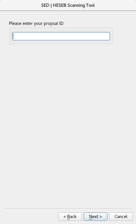
Figure 2: upon choosing Users Experiment, you will be asked to provide scheduled proposal ID

By choosing “Users Experiment”, the scan tool will: * Ask you to provide the proposal number. * Validate whether the provided proposal number is correct and valid for this beam time. * If the validation result is okay, the tool will import the proposal metadata and include them in the experimental file. If not, user will be alerted!!

Note

The scanning tool is already integrated with the users database. All validation and metadata importing processes are done through such integration.

On the other hand, choosing Local Experiment is meant for beamline scientist to run InHouse research experiments.

Error

Users with scheduled beamtime are requested to choose Users Experiment in order to keep their experimental data consistent with the proposal metadata.

The scanning tool allows you to either enter new configuration and thus generate a new configuration file or load already exist configuration file. These two options can be chosen from this GUI:

Figure 3: config choosing GUI, either to create new config file or load already existed one

Next GUI is meant to enter new experiment configurations or see/edit a loaded one. This GUI allows you to move the energy over a range by driving the theta motor of the Double Crystal Monochromator (DCM).

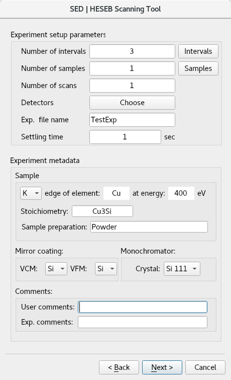
Figure 4: Main configuration GUI

The user can enter many intervals, each interval has start energy (eV), end energy (eV), energy move step size (eV) and integration time of the picoAmmeters.

Figure 5: Ranges across intervals

You can define many samples and align them with respect to the beam (depending on the number of holders installed on the sample stage). Through this GUI you can change the sample position horizontally and vertically in order to target the right position of the sample. Also, for each sample you must assign name where it will be used as part of the experimental file name.

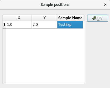
Figure 6: sample position and name

Note

sample name is added as part of the experimental file name

Detectors popup window allows you to choose among the available transmission and florescence detectors, I0 (PicoAmmeter1) is already chosen by default all the time, the possible choices are:

• I0

• I0 and Itrans

• I0, Itrans and Bruker XFlash

• I0 and Bruker XFlash

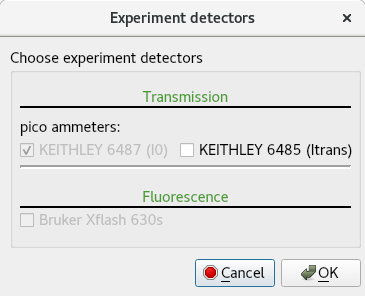
Figure 7: detectors choosing window

Note

Bruker XFlash detector is disabled because it is not yet integrated with the scanning tool

Other scan parameters in the main confirmation GUI like “Experiment metadata”, “Mirror coating” and “Comments” are used to provide some experimental meta data.

Note

Some experiment metadata fields are mandatory because they are needed to comply with xdi file format.

By clicking “Next”, if all is fine, the last GUI will pop up as shown below:

Figure 8: Last GUI, ready to start the scan

Once scan is started, interactive logs will be printed on the terminal showing exactly what is being processed. Also, an interactive data visualization tool will start plotting the experimental data.

Figure 9: data visualization of the experimental data

The interactive data visualization tool of the experimental data is devided to three sections:

1. Monitoring section

2. Control section

3. Plotting section

As shown in the figure.10, the main information about the monitoring section are:

• Start time: experiment starting time.

• Elapsed time: elapsed time for each sample.

• Sample # out of #: experiment samples.

• Scans # out of #: experiment scans.

• Intervals # out of #: experiment intervals.

• Sample X: the position of sample X.

• Sample Y: the position of sample Y.

• Energy (eV): the current energy of the beamline.

• Scan tool status: the logs and information of the experiment.

The main functions about the control section are:

• Pause: pasuse the scan.

• Resume: resume the scan.

• Stop: stop the scan.

• SED Path: the directory of the experiment.

• BL Parameters: a split GUI is developed to monitor the status of the beamline’s front end, optics, ID, and other components, as shown in the figure.10:

  • Source:

    1. C: Machine Current

    2. UG: Undulator Gap

    3. US: Undulator Shift

    4. UPSX: Upstram BPM (10;4)X

    5. UPSY: Upstram BPM (10;4)Y

    6. DWSX: Upstram BPM (11;1)X

    7. DWSY: Upstram BPM (11;1)Y

  • Mirrors(1, 3, 4a):

    1. R: Roll

    2. P: Pitch

    3. Y: Yaw

    4. HT: Horizontal Translation

    5. VT: Vertical Translation

    6. CP: Chamber Position

  • Movable Masks:

    1. HG: Horizontal Gap

    2. VG: Vertical Gap

    3. HC: Horizontal Center

    4. VC: Vertical Center

  • Vertical Slit:

    1. VS: Vertical Slit Width

  • Scan Parameters:

    1. C: Magnification Magnitude

    2. K: Diffraction Order

    3. G: Grating

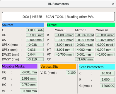
Figure 10: Beamline Parameters

The main information about the plotting section are:

• plotting the energy (eV) of the beamline vs. pico ammeter current acquired (A).

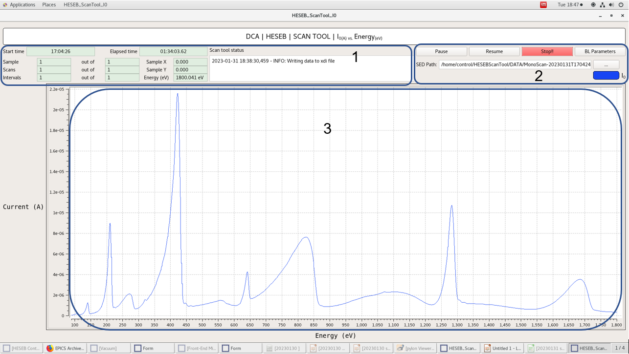
Figure 11: data visualization Tool

Live Data Plotting

Live data collection by countinuous moving of PGM depending on predefined integration time.

The live data plotting tool is located in the home directory of the control user. To access it:

$ HESEB_ScanTool_LiveDataVisualization

The main GUI will appear as shown in figure.12:

Figure 12: Live Data Visualization Tool

The main buttons and status labels are:

• I0: open (I0 vs Time) collection tool.

• It: open (It vs Time) collection tool.

• help: open the GUI documentation.

• status labels: running >> In Process… , not running >> Stopped

After selection, the main visualization tool will appear as shown in figure.13.

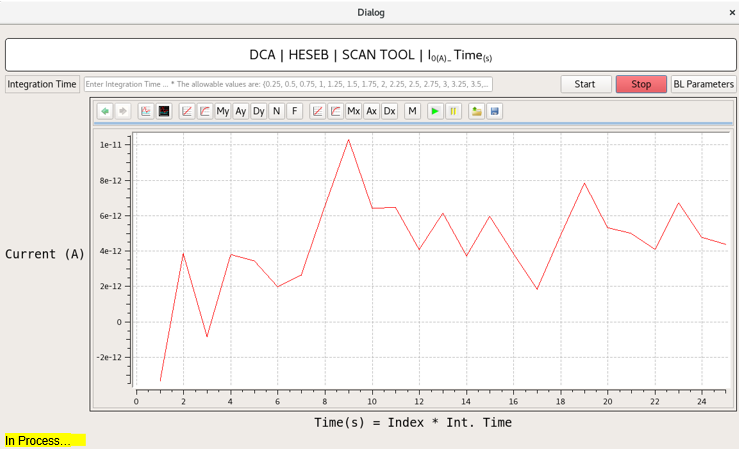
Figure 13: Live Data Plotting

The live data plotting is tool devided to:

1. Control section

2. Plotting section

As shown in the previous figure, the main functions of the control section are:

• integration Time: user input, based on specific values.

• Start: start collection.

• Stop: stop collection.

The main functions of the plotting section are:

• previous state.

• next state.

• white background.

• black background.

• linear scale of Y-axis.

• log scale of Y-axis.

• My: manual scale of Y-axis.

• Ay: data range of Y-axis.

• Dy: dynamic scale of Y-axis.

• N: normalized scale.

• F: fractional scale.

• linear scale of X-axis.

• log scale of X-axis.

• Mx: manual scale of X-axis.

• Ax: data range of X-axis.

• Dx: dynamic scale of X-axis.

• M: manual scale of X-Y axes.

• play -real time-.

• pause.

• load configurations.

• save configurations.